Fourier Series, Parseval’s Identity, and \(\zeta(2)\)

This post is inspired by a lecture series given by David Skinner in 2016. In particular, for further reading on Fourier series, see chapter 1 of the Mathematical Methods lecture notes.

Vector Spaces and Inner Products

Recall that a vector space over a field \(\mathbb F\) (in this post, always \(\mathbb R\) or \(\mathbb C\)) is a set \(V\) with an operation \(+ : V^2 \to V\) (commutative, associative, and with an identity \(0 \in V\)), with multiplication by elements of \(\mathbb F\) that is distributive in both \(V\) and \(F\),

\[c (\mathbf u + \mathbf v) = c \mathbf u + c \mathbf v \quad \forall c \in \mathbb F, \; \mathbf u, \mathbf v \in V\] \[(c_1 + c_2) \mathbf v = c_1 \mathbf v + c_2 \mathbf v \quad \forall c_1, c_2 \in \mathbb F, \; \mathbf v \in V\]

The most common example of a vector space is that of \(\mathbb R^n\) (over \(\mathbb R\)), which are \(n\)-tuples of real numbers. Recall that for such a space, we have a dot product

\[\mathbf u \cdot \mathbf v = \sum_i u_i v_i\]

Note that similarly, \(\mathbb C^n\) forms a vector space with a compatible dot product

\[\mathbf u \cdot \mathbf v = \sum_i \overline{u_i} v_i\]

where \(\overline{z}\) is the complex conjugate of the complex number \(z\).

Inner Products

The dot products on these spaces are examples of inner products, which are functions \(V^2 \to \mathbb F\), often denoted by parentheses \((\mathbf u, \mathbf v)\), such that it obeys:

• Conjugate symmetry: \((\mathbf u, \mathbf v) = \overline{(\mathbf{v}, \mathbf{u})}\)
• Linearity over \(\mathbb F\) in the second argument: \((\mathbf u, c \mathbf v) = c (\mathbf u, \mathbf v)\)
• Linearity over \(V\): \((\mathbf u, \mathbf v_1 + \mathbf v_2) = (\mathbf u, \mathbf v_1) + (\mathbf u, \mathbf v_2)\)
• Positive definiteness: \((\mathbf v, \mathbf v) \geq 0\), with \((\mathbf v, \mathbf v) = 0 \iff \mathbf v = \mathbf 0\)

Note that the first two conditions combined imply that \((c \mathbf u, \mathbf v) = \overline{c} (\mathbf u, \mathbf v)\).

One can check that the dot products mentioned above satisfy these requirements and are therefore inner products. We say that \(V\) equipped with this inner product is an inner product space. Due to the positive definiteness property, we can introduce a concept of a length,

\[\| \mathbf v \| = \sqrt{(\mathbf v, \mathbf v)}\]

which in the case of \(\mathbb R^n\) with the standard inner product becomes the usual Euclidean norm

\[\| (v_1, \dots, v_n) \| = \sqrt{\sum_i v_i^2}\]

Bases

In the finite dimensional case, we say that a set \(\mathcal B = \lbrace \mathbf e_1, \dots, \mathbf e_n \rbrace\) forms a basis for \(V\) if every element \(\mathbf v \in V\) can be expressed as a unique linear combination of elements in \(\mathcal B\). We then say that \(n\) is the dimension of \(V\).

For example, in \(\mathbb R^n\), if we define

\[\mathbf e_i = \underbrace{(0, \dots, 0, 1, 0, \dots, 0)}_{1\text{ in the } i^\text{th} \text{ place}}\]

then every vector \(\mathbf r = (r_1, r_2, \dots r_n) \in \mathbb R^n\) can be written as

\[\mathbf r = \sum_i r_i \mathbf e_i\]

and hence \(\mathcal B = \lbrace \mathbf e_i : i = 1, \dots, n \rbrace\) forms a basis for \(\mathbb R^n\).

Furthermore, we say that a set of vectors \(\mathcal O = \lbrace \mathbf v_1, \dots, \mathbf v_m \rbrace\) for some \(m \in \mathbb N\) is orthogonal if

\[(\mathbf v_i, \mathbf v_j) = 0 \; \forall i \neq j\]

and is orthonormal if each \(\mathbf v_i\) is of unit length, so that the above becomes

\[(\mathbf v_i, \mathbf v_j) = \delta_{ij}, \quad i, j \in \lbrace 1, \dots, m \rbrace\]

where we’ve introduced the usual Kronecker delta

\[\delta_{ij} = \begin{cases} 1 & i = j \\ 0 & \text{otherwise} \end{cases}\]

Note that for orthonormal bases, the components of a vector with respect to a given basis are simply the inner products, since

\[\begin{align} (\mathbf e_i, \mathbf r) &= \left( \mathbf e_i, \sum_j r_j \mathbf{e}_j \right) \\ &= \sum_j \left( \mathbf e_i, r_j \mathbf{e}_j \right) && \text{by linearity over } V\\ &= \sum_j r_j \left( \mathbf e_i, \mathbf{e}_j \right) && \text{by linearity over } \mathbb F \text{ in the second argument} \\ &= \sum_j r_j \delta_{ij} && \text{since the } \lbrace\mathbf e_i\rbrace \text{ are orthonormal} \\ &= r_i \end{align}\]

That is,

\[\mathbf r = \sum_i (\mathbf e_i, \mathbf r) \, \mathbf e_i\]

Infinite Dimensional Vector Spaces

Observe how in the definition of a vector space, despite calling elements of \(V\) vectors, we never required that they must be what we traditionally refer to as “vectors” - that is, elements of \(\mathbb R^n\) (or \(\mathbb C^n\)). In particular, let’s now consider the set

\[V = \lbrace f : f \text{ is a function } \mathbb R \to \mathbb R \rbrace\]

This forms a vector space over \(\mathbb R\) if we define the following:

• \(0\) is the zero function \(x \mapsto 0\)
• \(f + g\) is the function defined by \((f + g)(x) = f(x) + g(x)\)
• \(cf\) for \(c \in \mathbb r\) is defined by \((cf)(x) = c \cdot f(x)\)

One can check that with these unsurprising definitions, \(V\) is indeed a vector space. Similarly, if we replace \(\mathbb R \to \mathbb C\) in the above, we also have a vector space (over either set).

We now wish to introduce an inner product on our vector space. If we view a function as a continuous analogy of a vector in \(\mathbb R^n\) so that each “component”, rather than being indexed by a natural number \(i\), is instead indexed by the real number \(x\), then one might naturally write down

\[(f, g) = \int_{-\infty}^\infty f(x) g(x) \; dx\]

This turns out to be essentially correct, except for the slight issue of well-definedness. In particular, not every function is integrable, and even perfectly well-behaved functions such as \(f(x) = x\) suffer from the problem of convergence,

\[(x, x) = \int_{-\infty}^\infty x^2 \; dx \to \infty\]

With an eye on our Fourier series destination in mind, we can swiftly resolve these two problems. For the second, we simply restrict to a finite interval of \(\mathbb R\) - for example, \([0, T]\) for some real number \(T > 0\). This is almost good enough, except we still have some misbehaving functions. For example, if we define

\[f(x) = \begin{cases} x^{-1} & x \neq 0 \\ 0 & \text{otherwise} \end{cases}\]

then

\[(f, f) = \int_0^T x^{-2} dx\]

which is not convergent. Here, we resort to simply abandoning all functions which are not square-integrable, and instead consider only the space

\[f \in L^2(I) \iff f : I \to \mathbb R \text{ with } \int_I \lvert f \rvert^2 dx < \infty\]

where \(I = [0, T]\) is our sub-interval of \(\mathbb R\) of interest.

Note that for complex-valued functions, the inner product of interest is given by

\[(f, g) = \int_I \bar{f} g \, dx\]

Orthogonal Bases

It should be clear that, with each element \(f \in L^2\) having infinitely many degrees of freedom (loosely, one for each real number \(x\)), that no finite basis will exist. But, following the path we took in the finite dimensional case, we would still like to try and find an orthogonal basis.

Let’s fix \(T = 2 \pi\), and define \(f_n : \mathbb R \to \mathbb C\) by

\[f_n(x) = e^{i n x}, \; n \in \mathbb Z\]

Then, suppose \(n \neq m\) and consider

\[\begin{align} (f_n, f_m) &= \int_0^{2 \pi} e^{-inx} e^{imx} \; dx \\ &= \int_0^{2 \pi} e^{i(m-n)x} \; dx \\ &= \frac{1}{i(m-n)} \left[ e^{i(m-n)x} \right]_{0}^{2 \pi} = 0 \end{align}\]

where, since \(m - n \in \mathbb Z\), both endpoints have the value \(1\).

The remaining case \(m = n\) is trivial, since

\[(f_n, f_n) = \int_0^{2 \pi} e^{-inx} e^{inx} \; dx = \int_0^{2 \pi} dx = 2 \pi\]

It follows that

\[(f_n, f_m) = 2 \pi \delta_{nm}\]

and hence, the \(\lbrace f_n \rbrace\) are orthogonal.

Moreover, if one chooses to rescale \(f_n \mapsto g_n = \frac{1}{\sqrt{2 \pi}} f_n\), then these rescaled functions are orthonormal.

Fourier Series

It turns out that if one restricts attention to suitably well-behaved functions, then it is possible to write (where the equality is not quite strict)

\[f(x) = \sum_{n \in \mathbb Z} c_n e^{\frac{2 \pi i n x}{T}}\]

and for such functions, this will hold for all points \(x\) where the original function \(f(x)\) is continuous. The sum on the RHS of this equality is known as the Fourier series of \(f\).

Fourier Coefficients

Note how we’ve re-introduced our interval length \(T\) (which was previously \(2 \pi\)). In order to make this \(T\) more concrete, when it comes to Fourier series, we often consider periodic functions \(f : \mathbb R \to \mathbb R\). We say a function is periodic with period \(T > 0\) if

\[f(t + T) = f(t) \; \forall t \in \mathbb R\]

and we generally take \(T\) to be the least such \(T\). In this case, the function is fully described by its values on any interval of length \(T\), and often we will take the interval to be either of \([0, T]\) or \([-T/2, T/2]\).

For example, the sawtooth function is given by the periodic extension of

\[\begin{align} f : [-\pi, \pi] &\to \mathbb R \\ t &\mapsto t \end{align}\]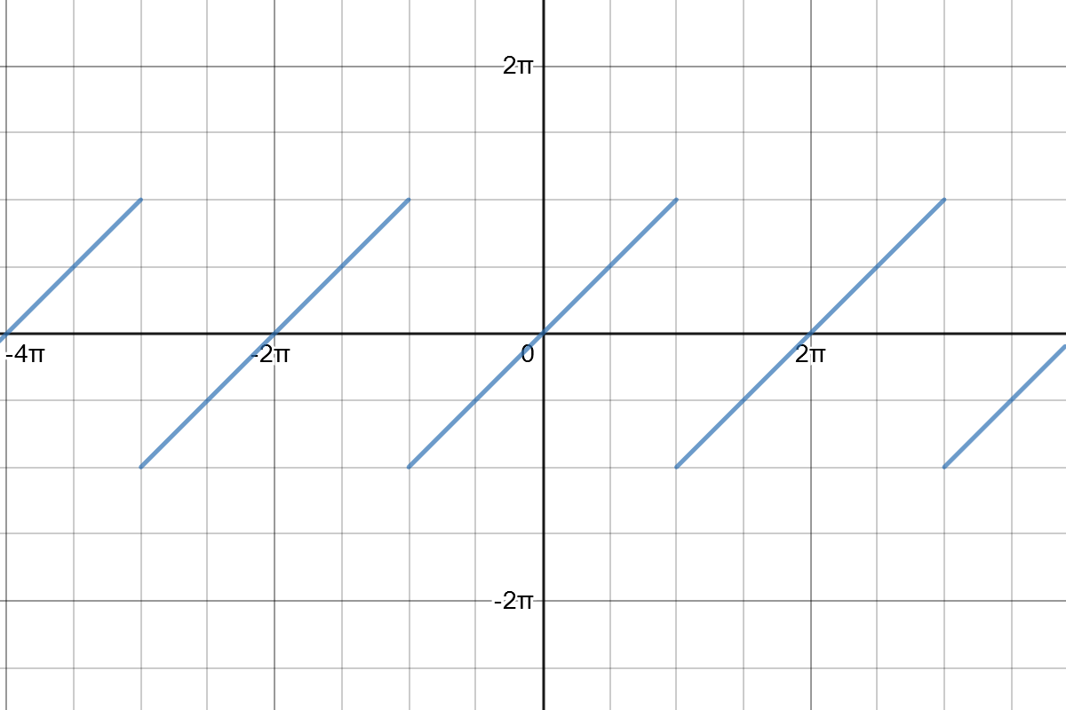

We then consider Fourier series on this interval, which, by periodicity, applies everywhere in \(\mathbb R\).

A sufficient set of conditions for the Fourier series of \(f\) (defined on \([0, T]\)) to agree with \(f\) at points where it is continuous are the Dirichlet conditions:

• \(f\) is bounded
• \(f\) has a finite number of minima, maxima, and discontinuities

Given that such a Fourier series exists, observe that

\[\begin{align} \left(e^\frac{2 \pi i m x}{T}, \; f(x)\right) &= \left(e^\frac{2 \pi i m x}{T}, \; \sum_{n \in \mathbb Z} c_n e^{\frac{2 \pi i n x}{T}}\right) \\ &= \sum_{n \in \mathbb z} c_n T \delta_{mn} = c_m T \end{align}\]

where we’ve implicitly assumed it is safe to exchange the order of the integration and the summation, so that we have

\[c_m = \frac{1}{T} \left(e^\frac{2 \pi i m x}{T}, f(x)\right)\]

which is directly analogous with the finite-dimensional case.

An Example

Return to the sawtooth function defined on \([-\pi, \pi]\),

\[f(\theta) = \theta\]

Its Fourier coefficients are given by

\[c_m = (e^{im \theta}, \theta) = \frac{1}{2 \pi} \int_{-\pi}^\pi e^{-im\theta} \theta \; d\theta\]

Observe that \(c_0 = 0\). For \(m \neq 0\), we expand the exponential as \(\cos m \theta - i \sin m \theta\) to obtain

\[\begin{align} c_m &= \frac{1}{2 \pi} \left( \underbrace{\int_{-\pi}^\pi \theta \cos m \theta \; d \theta}_{0 \text{ by parity}} - \int_{-\pi}^{\pi} i \theta \sin m \theta \; d \theta \right) \\ &= -\frac{i}{\pi} \int_0^\pi \theta \sin m \theta \; d\theta && \text{since the integrand is even}\\ &= -\frac{i}{\pi} \left( \left[ \frac{-\theta \cos m \theta}{m} \right]_0^\pi + \int_0^\pi \frac{\cos m \theta}{m} \; d\theta \right) && \text{integrating by parts} \\ &= \frac{i \cos \pi m}{m} - \frac{i}{\pi} \underbrace{\left[\frac{\sin m \theta}{m^2}\right]_0^\pi}_{0} && \text{by parts again}\\ &= \frac{(-1)^m i}{m} \end{align}\]

and hence we obtain the following Fourier series for \(f(\theta)\),

\[i \sum_{n \in \mathbb Z \\ n \neq 0} \frac{(-1)^n e^{i n \theta}}{n}\]

Note that the imaginary part necessarily vanishes, which we can observe by rewriting the sum as

\[\begin{align} \sum_{n \in \mathbb N} (-1)^n i \left[\frac{e^{i n \theta}}{ n} - \frac{e^{-i n \theta}}{n} \right] &= 2 \sum_{n \in \mathbb N} \frac{(-1)^{n+1}}{n} \frac{e^{i n \theta} - e^{-in\theta}}{2i} \\ &= 2 \sum_{n \in \mathbb N} \frac{(-1)^{n + 1}}{n} \cdot \sin n \theta \end{align}\]

Parseval’s Identity

A useful result, known as Parseval’s Identity, can be derived by considering the following:

\[\begin{align} (f, f) &= \left( \sum_n c_n e^{\frac{2 \pi n x}{T}}, \sum_m c_m e^{\frac{2 \pi m x}{T}} \right) \\ &= \sum_{n, m} \overline{c_n} c_m \underbrace{\left( e^{\frac{2 \pi n x}{T}}, e^{\frac{2 \pi m x}{T}} \right)}_{T \delta_{nm}} \\ &= T \sum_n \lvert c_n \rvert^2 \end{align}\]

The usefulness of this comes by noting that often, we can evaluate this directly using the integral

\[(f, f) = \int_0^T \lvert f(t) \rvert^2 \, dt\]

and hence we obtain the equality

\[\frac{1}{T} \int_0^T \lvert f(t) \rvert^2 \, dt = \sum_n \lvert c_n \rvert^2\]

where the \(c_n\) are the Fourier coefficients of \(f\). This is a useful trick for finding values of infinite series.

Applying Parseval’s identity to the sawtooth function above, we find that

\[\sum_n \lvert c_n \rvert^2 = \sum_{n \in \mathbb Z \\ n \neq 0} \frac{1}{n^2} = 2 \sum_{n=1}^\infty \frac{1}{n^2}\]

Evaluating the integral, we then find

\[\frac{1}{T} \int_{-\pi}^\pi \lvert f(t) \rvert^2 \, dt = \frac{1}{2 \pi} \int_{-\pi}^{\pi} t^2 \, dt = \frac{1}{6 \pi} \cdot 2 \pi^3 = \frac{\pi^2}{3}\]

and hence, applying Parseval’s Identity, we deduce that

\[2 \sum_{n=1}^\infty \frac{1}{n^2} = \frac{\pi^2}{3} \implies \sum_{n=1}^\infty \frac{1}{n^2} = \frac{\pi^2}{6}\]

This is a neat way to derive the value of \(\zeta(2)\), a result known as the Basel problem. Similarly, it is possible to derive values of \(\zeta(2k)\) by considering the Fourier series of \(\theta^k\). Deducing exact constants is somewhat tedious for \(k > 2\), but an inductive argument can be used to show that all such values of \(\zeta\) are rational multiples of powers of \(\pi\).